Table Of Content
But B appears not to be important either as a main effect or within any interaction. B was the rate of gas flow across the edging process and it does not seem to be an important factor in this process, at least for the levels of the factor used in the experiment. The difference between red and green bars is small for level 1 of IV1, but large for level 2. The differences between the differences are different, so there is an interaction. For example, both the red and green bars for IV1 level 1 are higher than IV1 Level 2. And, both of the red bars (IV2 level 1) are higher than the green bars (IV2 level 2).
Data Requirements
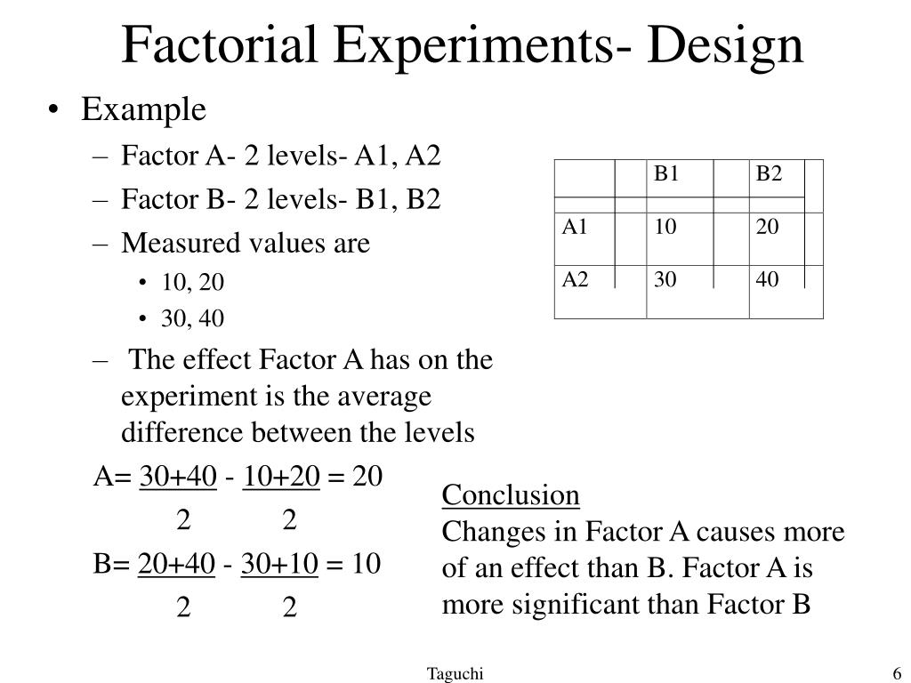
The research designs we have considered so far have been simple—focusing on a question about one variable or about a relationship between two variables. In this chapter, we look closely at how and why researchers use factorial designs, which are experiments that include more than one independent variable. In the middle panel, independent variable “B” has a stronger effect at level 1 of independent variable “A” than at level 2. This is like the hypothetical driving example where there was a stronger effect of using a cell phone at night than during the day. In the bottom panel, independent variable “B” again has an effect at both levels of independent variable “A”, but the effects are in opposite directions. One example of a crossover interaction comes from a study by Kathy Gilliland on the effect of caffeine on the verbal test scores of introverts and extraverts [Gil80].
Experimental Design – Types, Methods, Guide
Full factorial designs grow large as the number of factors increases, but we can use fractional factorial designs to reduce the number of runs required by considering only a fraction of the full factorial runs (e.g., half as many in a 26–1 design). These runs are chosen carefully so that under the reasonable assumptions of effect sparsity and hierarchy, the terms of interest (e.g., main effects and two-factor interactions) can be estimated. In addition to looking at the employment sector, the researchers also look at gender. In this example, the employment sector and gender of the graduates are the independent variables, and the starting salaries are the dependent variables.
What Are Factorial Experiments and Why Can They Be Helpful?
For instance, if the purity, yield, and residual amount of catalyst was measured in the DOE study, the values of these for each trial would be entered in the columns. In the "Modify Design" menu, users can modify factors, replicate design, randomize design, renumber design, fold design, and add axial points. To change the factors, click the "Modify factors" radio button and then "Specify" to see the following options menu.
Minitab DOE Example
Complex correlational research, however, can often be used to rule out other plausible interpretations. Importantly, the effect of the gas variable on driving depends on the levels of having a key. Or, to state it in reverse, the effect of the key variable on driving depends on the levesl of the gas variable. Except in this case, we find the average heights in the no hat vs. hat conditions by averaging over the shoe variable. Other options can be selected from the "Analyze Factorial Design" menu such as "Covariates...", "Prediction...", "Storage...", and "Weights...".
Full factorial design and dynamic modelling of silent and ultrasound-assisted lead and cadmium removal by porous ... - Nature.com
Full factorial design and dynamic modelling of silent and ultrasound-assisted lead and cadmium removal by porous ....
Posted: Thu, 28 Apr 2022 07:00:00 GMT [source]
It is particularly useful when studying the impact of an intervention or treatment on a particular outcome. Factor analysis is used to identify underlying factors or dimensions in a set of variables. This can be used to reduce the complexity of the data and identify patterns in the data. Descriptive statistics are used to summarize and describe the data collected in the study. This includes measures such as mean, median, mode, range, and standard deviation. This involves systematically varying the order in which participants receive treatments or interventions in order to control for order effects.
The coefficients and constants for wt% methanol in biodiesel and number of theoretical stages are shown below. In the main "Create Factorial Design" menu, click "OK" once all specifications are complete. The following table is obtained for a 2-level, 4 factor, full factorial design. None of the levels were specified as they appear as -1 and 1 for low and high levels, respectively.
3.2. Main effects
An interaction is a result in which the effects of one experimental manipulation depends upon the experimental manipulation of another independent variable. These equations can be used as a predictive model to determine wt% methanol in biodiesel and number of theoretical stages achieved at different operating conditions without actually performing the experiments. However, the limits of the model should be tested before the model is used to predict responses at many different operating conditions. In addition to the above effects plots, Minitab calculates the coefficients and constants for response equations. The response equations can be used as models for predicting responses at different operating conditions (factors).
V. Chapter 5: Experimental Research
Including additional factors in an experiment might certainly affect the significance tests of a given factor. The reduction in power will be greater if we control experiment-wise error, due to the larger number of main and interaction effects. Including numerous factors might also increase the occurrence of interactions, which might affect the magnitude of a main effect (despite the lack of correlation between main and interaction effects with effect coding). Most complex correlational research, however, does not fit neatly into a factorial design.
The research designs we have considered so far have been simple—focusing on a question about one variable or about a statistical relationship between two variables. But in many ways, the complex design of this experiment undertaken by Schnall and her colleagues is more typical of research in psychology. Fortunately, we have already covered the basic elements of such designs in previous chapters.
So, just looking at this summary information wouldn't tell us what to do except that we could drop the 3-way interaction. Let’s name our factors A, B and C, and use –1 and +1 for the low and high levels, respectively (Table 1). Even though there is no replication, this 23 full factorial design can detect factor effects, if some sensible assumptions are made. The researchers then decided to look at three levels of sleep (4 hours, 6 hours, and 8 hours) and only two levels of caffeine consumption (2 cups versus no coffee). The researchers note that the effects of the memory drug are more pronounced with the simple memory tasks, but not as apparent when it comes to the complex tasks. In this 3×2 factorial design, there is an interaction effect between the drug dosage and the complexity of the memory task.
More specifically, in both cases, wearing a hat adds exactly 6 inches to the height, no more no less. Make plots to determine the main or interaction effects of each factor. Suppose that you are looking to study the effects of hours slept (A), hours spent with significant other (B), and hours spent studying (C) on a students exam scores. You are given the following table that relates the combination of these factors and the students scores over the course of a semester. Use the Yates method in order to determine the effect each variable on the students performance in the course. The Pareto charts show which factors have statistically significant effects on the responses.
Just by virtue of doing separate studies, the opportunity for increased variability is introduced. The expectation in conducting randomized trials is that results can vary from study to study even when the designs are similar. The fact that the studies were conducted sequentially allows for further variability due to calendar time. It may be that neither of these sources of variability would be meaningful for these studies, but the design does not allow disaggregation of these extraneous features. The timing of the administration of light flashes (starting 3 hours before wake time in study 1 vs 2 hours before wake time in study 2) also changed.
We do have to take into account that these actual p-values are not something that you would consider very reliable because you are fitting this sequence of models, i.e., fishing for the best model. We have optimized with several decisions that invalidates the actual p-value of the true probability that this could have occurred by chance. In these experiments one really cannot model the "noise" or variability very well. These experiments cannot really test whether or not the assumptions are being met - again this is another shortcoming, or the price of the efficiency of these experiment designs. To restate this, in terms of A, the A effect is the difference between the means at the high levels of A versus the low levels of A, whereas the coefficient, \(\alpha_i\), in the model is the difference between the marginal mean and the overall mean. So the Yates "effect" is twice the size of the estimated coefficient αi in the model, which is also usually called the effect of factor A.

No comments:
Post a Comment